Data acquisition with PyUL
| Date: | 2018-12-12 (last modified), 2006-11-06 (created) |
|---|
Introduction
This pages illustrates the use of the inexpensive (about \$190) PMD USB-1208FS data acquisition device from Measurement Computing. It makes use of PyUniversalLibrary, an open-source wrapper of Measurement Computing's Universal Library.
See also Data acquisition with Ni-DAQmx.
The following examples were made with PyUL Release 20050624. The pre-compiled win32 binaries of this version are compatible with the Enthought Edition of Python 2.4 (Release 1.0.0, 2006-08-02 12:20), which is what was used to run these examples.
Example 1 - Simple Analog input
The first example illustrates the use of the unbuffered analog input:
# example1.py
import UniversalLibrary as UL
import time

BoardNum = 0
Gain = UL.BIP5VOLTS
Chan = 0

tstart = time.time()
data = []
times = []
while 1:
    DataValue = UL.cbAIn(BoardNum, Chan, Gain)
    data.append( DataValue )
    times.append( time.time()-tstart )
    if times[-1] > 1.0:
        break

import pylab
pylab.plot(times,data,'o-')
pylab.xlabel('time (sec)')
pylab.ylabel('ADC units')
pylab.show()
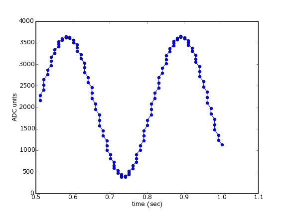
When I ran this, I had a function generator generating a sine wave connected to pins 1 and 2 of my device. This should produce a figure like the following:

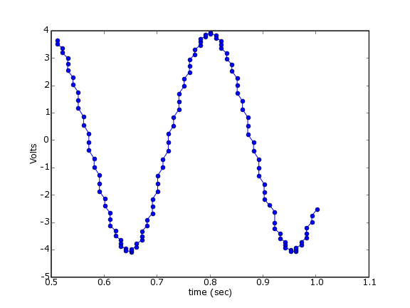
Example 2 - Getting Volts rather than arbitrary units
The values recorded in example 1 are "ADC units", the values recorded directly by the Analog-to-Digital hardware. In fact, this device has a 12-bit A to D converter, but the values are stored as 16-bit signed integers. To convert these values to Volts, we use Measurement Computing's function. Here we do that for each piece of data and plot the results.
#example2.py
import UniversalLibrary as UL
import time

BoardNum = 0
Gain = UL.BIP5VOLTS
Chan = 0

tstart = time.time()
data = []
times = []
while 1:
    DataValue = UL.cbAIn(BoardNum, Chan, Gain)
    EngUnits = UL.cbToEngUnits(BoardNum, Gain, DataValue)
    data.append( EngUnits )
    times.append( time.time()-tstart )
    if times[-1] > 1.0:
        break

import pylab
pylab.plot(times,data,'o-')
pylab.xlabel('time (sec)')
pylab.ylabel('Volts')
#pylab.savefig('example2.png',dpi=72)
pylab.show()
Now the output values are in volts:
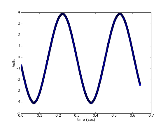
Example 3 - Buffered input
As you have no doubt noticed, the plots above aren't very "pure" sine waves. This is undoubtedly due to the way we're sampling the data. Rather than relying on a steady clock to do our acquisition, we're simply polling the device as fast as it (and the operating system) will let us go. There's a better way - we can use the clock on board the Measurement Computing device to acquire a buffer of data at evenly spaced samples.
#example3.py
import UniversalLibrary as UL
import Numeric
import pylab

BoardNum = 0
Gain = UL.BIP5VOLTS

LowChan = 0
HighChan = 0

Count = 2000
Rate = 3125

Options = UL.CONVERTDATA
ADData = Numeric.zeros((Count,), Numeric.Int16)

ActualRate = UL.cbAInScan(BoardNum, LowChan, HighChan, Count,
                      Rate, Gain, ADData, Options)

# convert to Volts
data_in_volts = [ UL.cbToEngUnits(BoardNum, Gain, y) for y in ADData]

time = Numeric.arange( ADData.shape[0] )*1.0/ActualRate

pylab.plot(time, data_in_volts, 'o-')
pylab.xlabel('time (sec)')
pylab.ylabel('Volts')
pylab.savefig('example3.png',dpi=72)
pylab.show()
The output looks much better: 
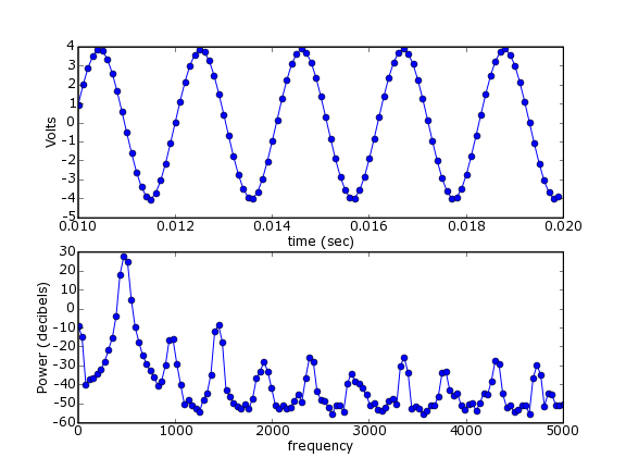
Example 4 - computing the power spectrum
Now we can use the function from pylab (part of matplotlib) to compute the power spectral density.
#example4.py
import UniversalLibrary as UL
import Numeric
import pylab

BoardNum = 0
Gain = UL.BIP5VOLTS

LowChan = 0
HighChan = 0

Count = 2000
Rate = 10000

Options = UL.CONVERTDATA
ADData = Numeric.zeros((Count,), Numeric.Int16)

ActualRate = UL.cbAInScan(BoardNum, LowChan, HighChan, Count,
                      Rate, Gain, ADData, Options)
time = Numeric.arange( ADData.shape[0] )*1.0/ActualRate

# convert to Volts
data_in_volts = [ UL.cbToEngUnits(BoardNum, Gain, y) for y in ADData]
data_in_volts = Numeric.array(data_in_volts) # convert to Numeric array

pxx, freqs = pylab.psd( data_in_volts, Fs=ActualRate )
decibels = 10*Numeric.log10(pxx)
pylab.subplot(2,1,1)
pylab.plot(time[100:200],data_in_volts[100:200],'o-') # plot a few samples
pylab.xlabel('time (sec)')
pylab.ylabel('Volts')
pylab.subplot(2,1,2)
pylab.plot(freqs, decibels, 'o-')
pylab.xlabel('frequency')
pylab.ylabel('Power (decibels)')
pylab.savefig('example4.png',dpi=72)
pylab.show()
For this example, I've turned up the frequency on the function generator to 480 Hz. You can see, indeed, that's what the psd() function tells us:
Section author: AndrewStraw, Chris Waigl
Attachments