Least squares circle
| Date: | 2011-03-22 (last modified), 2011-03-19 (created) |
|---|
Introduction
This page gathers different methods used to find the least squares circle fitting a set of 2D points (x,y).
The full code of this analysis is available here: least_squares_circle_v1d.py.
Finding the least squares circle corresponds to finding the center of the circle (xc, yc) and its radius Rc which minimize the residu function defined below:
#! python
Ri = sqrt( (x - xc)**2 + (y - yc)**2)
residu = sum( (Ri - Rc)**2)
This is a nonlinear problem. We well see three approaches to the problem, and compare there results, as well as their speeds.
Using an algebraic approximation
As detailed in this document this problem can be approximated by a linear one if we define the function to minimize as follow:
#! python
residu_2 = sum( (Ri**2 - Rc**2)**2)
This leads to the following method, using linalg.solve :
#! python
# == METHOD 1 ==
method_1 = 'algebraic'

# coordinates of the barycenter
x_m = mean(x)
y_m = mean(y)

# calculation of the reduced coordinates
u = x - x_m
v = y - y_m

# linear system defining the center (uc, vc) in reduced coordinates:
#    Suu * uc +  Suv * vc = (Suuu + Suvv)/2
#    Suv * uc +  Svv * vc = (Suuv + Svvv)/2
Suv  = sum(u*v)
Suu  = sum(u**2)
Svv  = sum(v**2)
Suuv = sum(u**2 * v)
Suvv = sum(u * v**2)
Suuu = sum(u**3)
Svvv = sum(v**3)

# Solving the linear system
A = array([ [ Suu, Suv ], [Suv, Svv]])
B = array([ Suuu + Suvv, Svvv + Suuv ])/2.0
uc, vc = linalg.solve(A, B)

xc_1 = x_m + uc
yc_1 = y_m + vc

# Calcul des distances au centre (xc_1, yc_1)
Ri_1     = sqrt((x-xc_1)**2 + (y-yc_1)**2)
R_1      = mean(Ri_1)
residu_1 = sum((Ri_1-R_1)**2)
Using scipy.optimize.leastsq
Scipy comes will several tools to solve the nonlinear problem above. Among them, scipy.optimize.leastsq is very simple to use in this case.
Indeed, once the center of the circle is defined, the radius can be calculated directly and is equal to mean(Ri). So there is only two parameters left: xc and yc.
Basic usage
#! python
#  == METHOD 2 ==
from scipy      import optimize

method_2 = "leastsq"

def calc_R(xc, yc):
    """ calculate the distance of each 2D points from the center (xc, yc) """
    return sqrt((x-xc)**2 + (y-yc)**2)

def f_2(c):
    """ calculate the algebraic distance between the data points and the mean circle centered at c=(xc, yc) """
    Ri = calc_R(*c)
    return Ri - Ri.mean()

center_estimate = x_m, y_m
center_2, ier = optimize.leastsq(f_2, center_estimate)

xc_2, yc_2 = center_2
Ri_2       = calc_R(*center_2)
R_2        = Ri_2.mean()
residu_2   = sum((Ri_2 - R_2)**2)
Advanced usage, with jacobian function
To gain in speed, it is possible to tell optimize.leastsq how to compute the jacobian of the function by adding a Dfun argument:
#! python
# == METHOD 2b ==
method_2b  = "leastsq with jacobian"

def calc_R(xc, yc):
    """ calculate the distance of each data points from the center (xc, yc) """
    return sqrt((x-xc)**2 + (y-yc)**2)

def f_2b(c):
    """ calculate the algebraic distance between the 2D points and the mean circle centered at c=(xc, yc) """
    Ri = calc_R(*c)
    return Ri - Ri.mean()

def Df_2b(c):
    """ Jacobian of f_2b
    The axis corresponding to derivatives must be coherent with the col_deriv option of leastsq"""
    xc, yc     = c
    df2b_dc    = empty((len(c), x.size))

    Ri = calc_R(xc, yc)
    df2b_dc[0] = (xc - x)/Ri                   # dR/dxc
    df2b_dc[1] = (yc - y)/Ri                   # dR/dyc
    df2b_dc    = df2b_dc - df2b_dc.mean(axis=1)[:, newaxis]

    return df2b_dc

center_estimate = x_m, y_m
center_2b, ier = optimize.leastsq(f_2b, center_estimate, Dfun=Df_2b, col_deriv=True)

xc_2b, yc_2b = center_2b
Ri_2b        = calc_R(*center_2b)
R_2b         = Ri_2b.mean()
residu_2b    = sum((Ri_2b - R_2b)**2)
#! python
(x - xc)**2 + (y-yc)**2 - Rc**2 = 0
Basic usage
This leads to the following code:
#! python
# == METHOD 3 ==
from scipy      import  odr

method_3 = "odr"

def f_3(beta, x):
    """ implicit definition of the circle """
    return (x[0]-beta[0])**2 + (x[1]-beta[1])**2 -beta[2]**2

# initial guess for parameters
R_m = calc_R(x_m, y_m).mean()
beta0 = [ x_m, y_m, R_m]

# for implicit function :
#       data.x contains both coordinates of the points (data.x = [x, y])
#       data.y is the dimensionality of the response
lsc_data  = odr.Data(row_stack([x, y]), y=1)
lsc_model = odr.Model(f_3, implicit=True)
lsc_odr   = odr.ODR(lsc_data, lsc_model, beta0)
lsc_out   = lsc_odr.run()

xc_3, yc_3, R_3 = lsc_out.beta
Ri_3 = calc_R([xc_3, yc_3])
residu_3 = sum((Ri_3 - R_3)**2)
Advanced usage, with jacobian functions
One of the advantages of the implicit function definition is that its derivatives are very easily calculated.
This can be used to complete the model:
#! python
# == METHOD 3b ==
method_3b  = "odr with jacobian"

def f_3b(beta, x):
    """ implicit definition of the circle """
    return (x[0]-beta[0])**2 + (x[1]-beta[1])**2 -beta[2]**2

def jacb(beta, x):
    """ Jacobian function with respect to the parameters beta.
    return df_3b/dbeta
    """
    xc, yc, r = beta
    xi, yi    = x

    df_db    = empty((beta.size, x.shape[1]))
    df_db[0] =  2*(xc-xi)                     # d_f/dxc
    df_db[1] =  2*(yc-yi)                     # d_f/dyc
    df_db[2] = -2*r                           # d_f/dr

    return df_db

def jacd(beta, x):
    """ Jacobian function with respect to the input x.
    return df_3b/dx
    """
    xc, yc, r = beta
    xi, yi    = x

    df_dx    = empty_like(x)
    df_dx[0] =  2*(xi-xc)                     # d_f/dxi
    df_dx[1] =  2*(yi-yc)                     # d_f/dyi

    return df_dx

def calc_estimate(data):
    """ Return a first estimation on the parameter from the data  """
    xc0, yc0 = data.x.mean(axis=1)
    r0 = sqrt((data.x[0]-xc0)**2 +(data.x[1] -yc0)**2).mean()
    return xc0, yc0, r0

# for implicit function :
#       data.x contains both coordinates of the points
#       data.y is the dimensionality of the response
lsc_data  = odr.Data(row_stack([x, y]), y=1)
lsc_model = odr.Model(f_3b, implicit=True, estimate=calc_estimate, fjacd=jacd, fjacb=jacb)
lsc_odr   = odr.ODR(lsc_data, lsc_model)    # beta0 has been replaced by an estimate function
lsc_odr.set_job(deriv=3)                    # use user derivatives function without checking
lsc_odr.set_iprint(iter=1, iter_step=1)     # print details for each iteration
lsc_out   = lsc_odr.run()

xc_3b, yc_3b, R_3b = lsc_out.beta
Ri_3b       = calc_R(xc_3b, yc_3b)
residu_3b   = sum((Ri_3b - R_3b)**2)
#! python
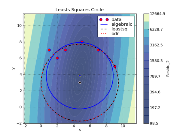
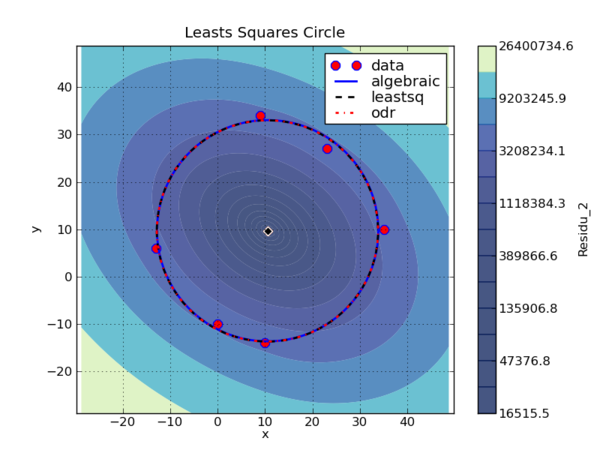
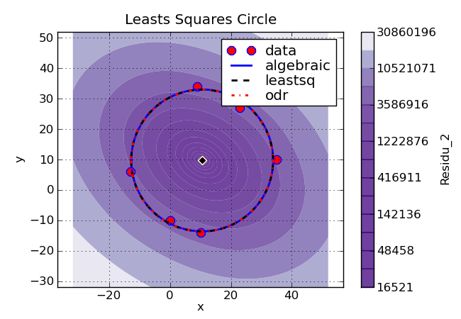
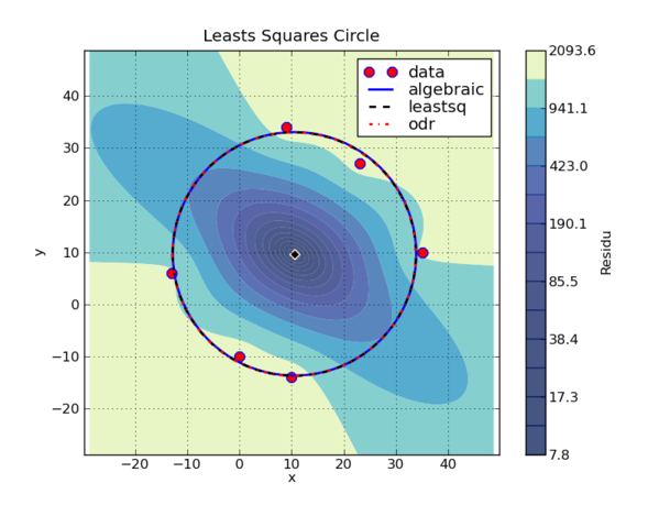
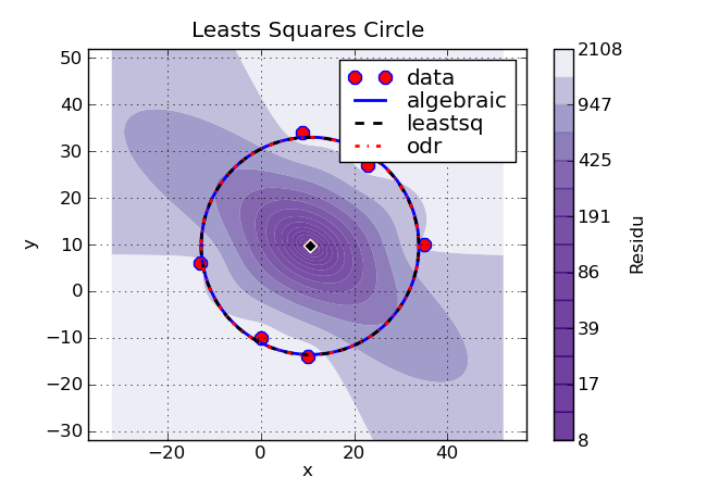
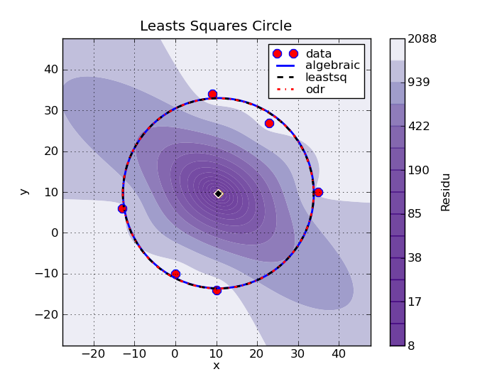
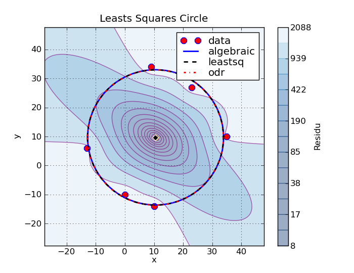
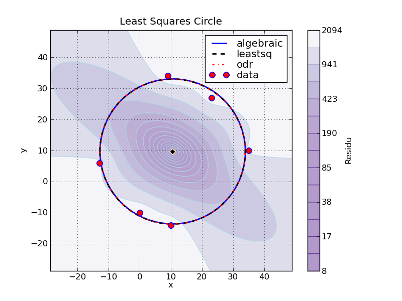
# Coordinates of the 2D points
x = r_[ 9, 35, -13, 10, 23, 0]
y = r_[ 34, 10, 6, -14, 27, -10]
This gives:
||||||||||||||||<tablewidth="100%">SUMMARY|| ||Method|| Xc || Yc || Rc ||nb_calls || std(Ri)|| residu || residu2 || ||algebraic || 10.55231 || 9.70590|| 23.33482|| 1|| 1.135135|| 7.731195|| 16236.34|| ||leastsq || 10.50009 || 9.65995|| 23.33353|| 15|| 1.133715|| 7.711852|| 16276.89|| ||leastsq with jacobian || 10.50009 || 9.65995|| 23.33353|| 7|| 1.133715|| 7.711852|| 16276.89|| ||odr || 10.50009 || 9.65995|| 23.33353|| 82|| 1.133715|| 7.711852|| 16276.89|| ||odr with jacobian || 10.50009 || 9.65995|| 23.33353|| 16|| 1.133715|| 7.711852|| 16276.89||
Note:
* `nb_calls` correspond to the number of function calls of the function to be minimized, and do not take into account the number of calls to derivatives function. This differs from the number of iteration as ODR can make multiple calls during an iteration.
* as shown on the figures below, the two functions `residu` and `residu_2` are not equivalent, but their minima are close in this case.


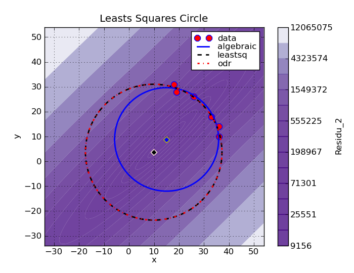
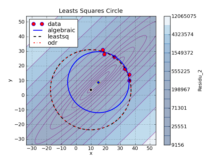
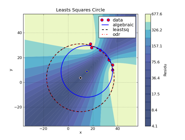
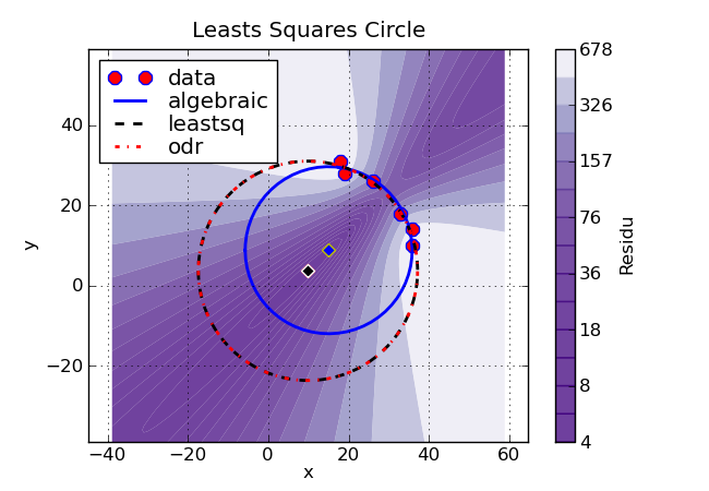
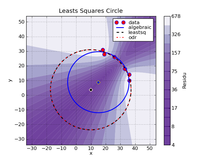
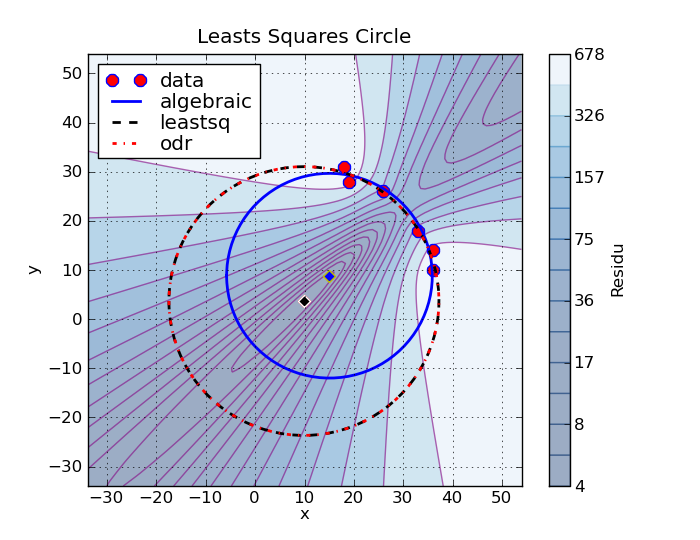
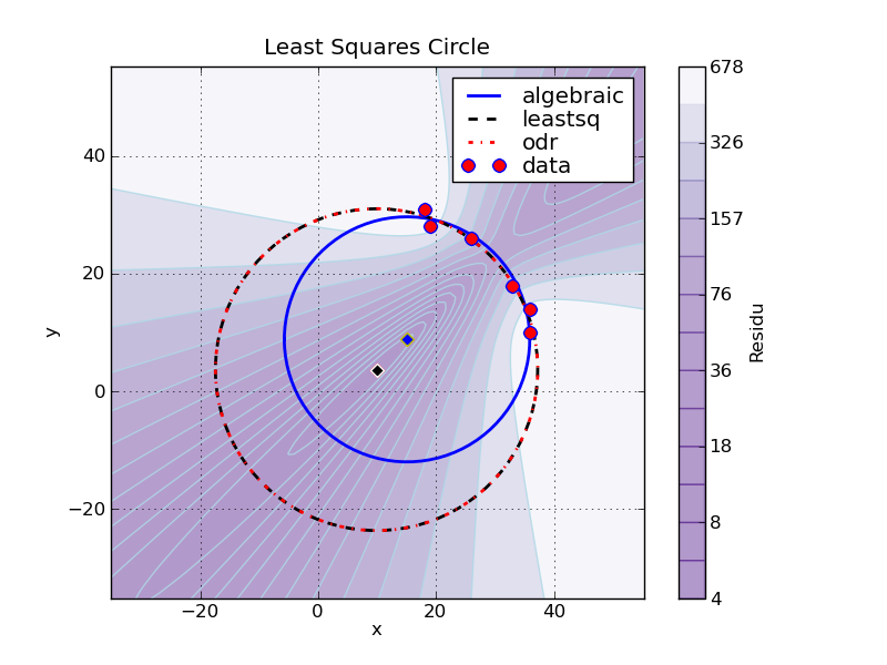
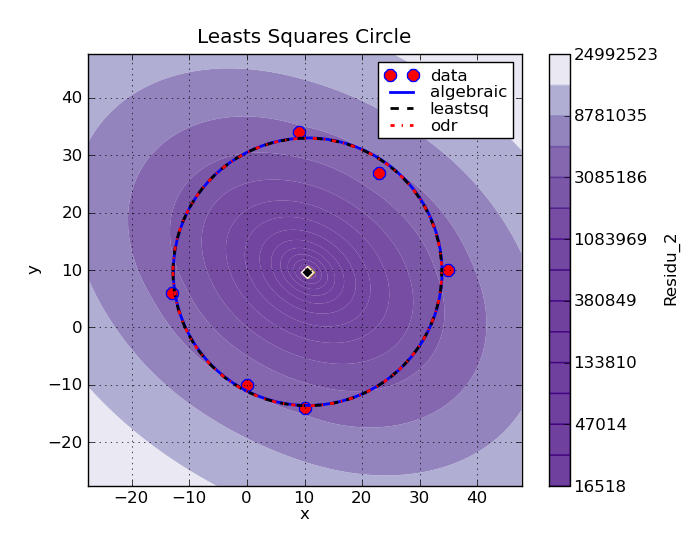
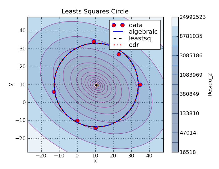
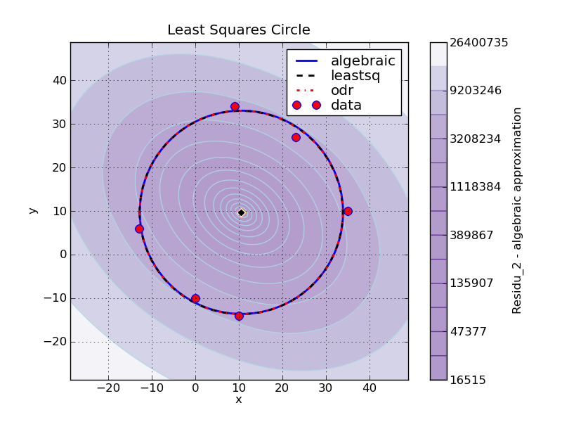
Data points around an arc
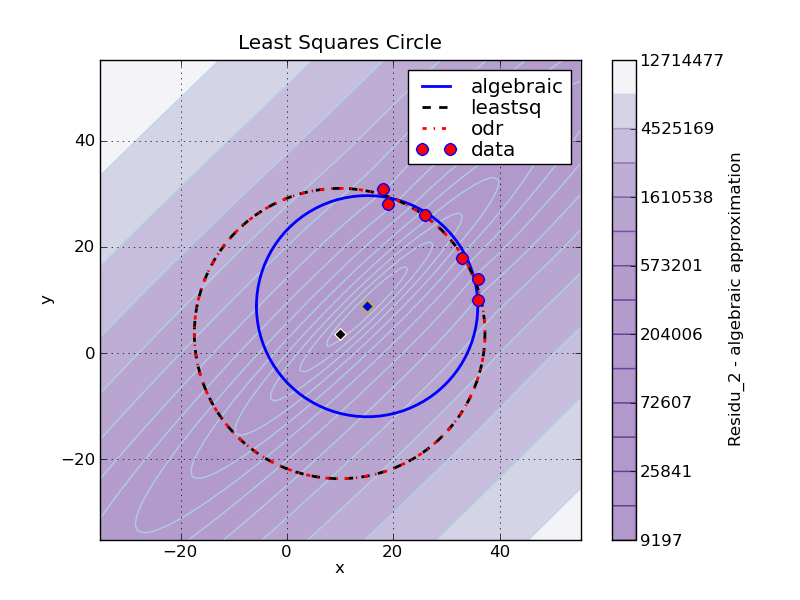
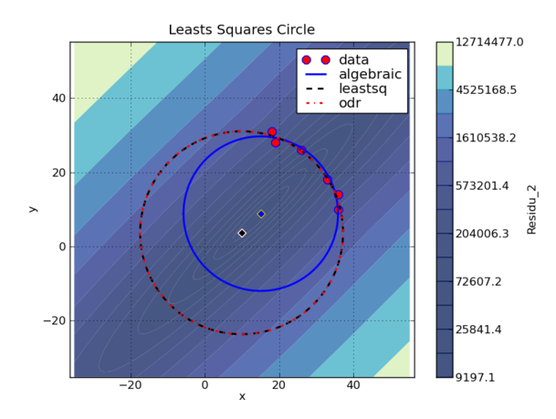
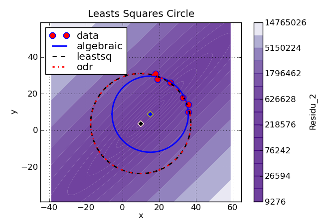
Here is an example where data points form an arc:
#! python
x = r_[36, 36, 19, 18, 33, 26]
y = r_[14, 10, 28, 31, 18, 26]
| '''Method''' | '''Xc''' | '''Yc''' | '''Rc''' | '''nb_calls''' | '''std(Ri)''' | '''residu''' | '''residu2''' |
|---|---|---|---|---|---|---|---|
| algebraic | 15.05503 | 8.83615 | 20.82995 | 1 | 0.930508 | 5.195076 | 9153.40 |
| leastsq | 9.88760 | 3.68753 | 27.35040 | 24 | 0.820825 | 4.042522 | 12001.98 |
| leastsq with jacobian | 9.88759 | 3.68752 | 27.35041 | 10 | 0.820825 | 4.042522 | 12001.98 |
| odr | 9.88757 | 3.68750 | 27.35044 | 472 | 0.820825 | 4.042522 | 12002.01 |
| odr with jacobian | 9.88757 | 3.68750 | 27.35044 | 109 | 0.820825 | 4.042522 | 12002.01 |
Conclusion
ODR and leastsq gives the same results.
Optimize.leastsq is the most efficient method, and can be two to ten times faster than ODR, at least as regards the number of function call.
Adding a function to compute the jacobian can lead to decrease the number of function calls by a factor of two to five.
In this case, to use ODR seems a bit overkill but it can be very handy for more complex use cases like ellipses.
The algebraic approximation gives good results when the points are all around the circle but is limited when there is only an arc to fit.
Indeed, the two errors functions to minimize are not equivalent when data points are not all exactly on a circle. The algebraic method leads in most of the case to a smaller radius than that of the least squares circle, as its error function is based on squared distances and not on the distance themselves.
Section author: Elby
Attachments
arc_residu2_v1.pngarc_residu2_v2.pngarc_residu2_v3.pngarc_residu2_v4.pngarc_residu2_v5.pngarc_residu2_v6.pngarc_v1.pngarc_v2.pngarc_v3.pngarc_v4.pngarc_v5.pngfull_cercle_residu2_v1.pngfull_cercle_residu2_v2.pngfull_cercle_residu2_v3.pngfull_cercle_residu2_v4.pngfull_cercle_residu2_v5.pngfull_cercle_v1.pngfull_cercle_v2.pngfull_cercle_v3.pngfull_cercle_v4.pngfull_cercle_v5.pngleast_squares_circle.pyleast_squares_circle_v1.pyleast_squares_circle_v1b.pyleast_squares_circle_v1c.pyleast_squares_circle_v1d.pyleast_squares_circle_v2.pyleast_squares_circle_v3.py