Using radial basis functions for smoothing/interpolation
| Date: | 2020-06-09 (last modified), 2007-02-08 (created) |
|---|
Radial basis functions can be used for smoothing/interpolating scattered data in n-dimensions, but should be used with caution for extrapolation outside of the observed data range.
1d example
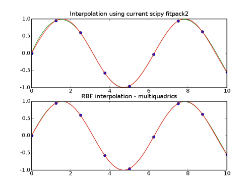
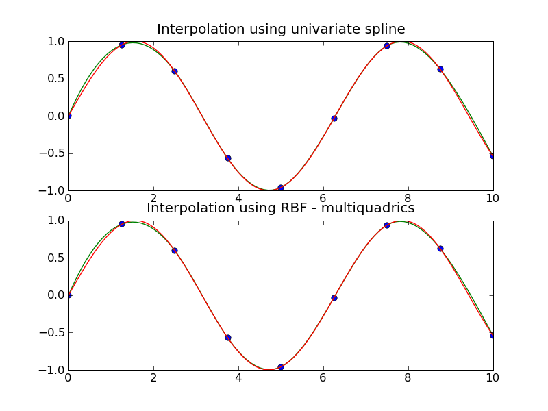
This example compares the usage of the Rbf and UnivariateSpline classes from the scipy.interpolate module.
In [ ]:
import numpy as np
from scipy.interpolate import Rbf, InterpolatedUnivariateSpline

import matplotlib
matplotlib.use('Agg')
import matplotlib.pyplot as plt

# setup data
x = np.linspace(0, 10, 9)
y = np.sin(x)
xi = np.linspace(0, 10, 101)

# use fitpack2 method
ius = InterpolatedUnivariateSpline(x, y)
yi = ius(xi)

plt.subplot(2, 1, 1)
plt.plot(x, y, 'bo')
plt.plot(xi, yi, 'g')
plt.plot(xi, np.sin(xi), 'r')
plt.title('Interpolation using univariate spline')

# use RBF method
rbf = Rbf(x, y)
fi = rbf(xi)

plt.subplot(2, 1, 2)
plt.plot(x, y, 'bo')
plt.plot(xi, fi, 'g')
plt.plot(xi, np.sin(xi), 'r')
plt.title('Interpolation using RBF - multiquadrics')
plt.tight_layout()
plt.savefig('rbf1d.png')

In [ ]:
import numpy as np
from scipy.interpolate import Rbf
import matplotlib
matplotlib.use('Agg')
import matplotlib.pyplot as plt
from matplotlib import cm
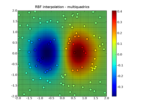
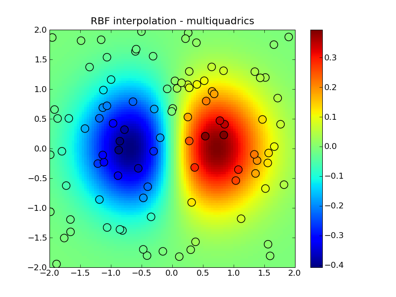
# 2-d tests - setup scattered data
x = np.random.rand(100)*4.0-2.0
y = np.random.rand(100)*4.0-2.0
z = x*np.exp(-x**2-y**2)
ti = np.linspace(-2.0, 2.0, 100)
XI, YI = np.meshgrid(ti, ti)
# use RBF
rbf = Rbf(x, y, z, epsilon=2)
ZI = rbf(XI, YI)
# plot the result
n = plt.normalize(-2., 2.)
plt.subplot(1, 1, 1)
plt.pcolor(XI, YI, ZI, cmap=cm.jet)
plt.scatter(x, y, 100, z, cmap=cm.jet)
plt.title('RBF interpolation - multiquadrics')
plt.xlim(-2, 2)
plt.ylim(-2, 2)
plt.colorbar()
plt.savefig('rbf2d.png')
Section author: Unknown[13], cassiasamp, Christian Gagnon
Attachments